Fractional Fourier Transform Continuous in Alpha
The Fourier Transform, outlined by French mathematician and physicist Joseph Fourier (1768-1830) in The Analytic Theory of Heat (1822), asserted that any function of a variable, whether continuous or discontinuous, can be expanded in a series of sines of multiples of the variable. His focus at the time was the propagation of heat in an iron ring, but in the next 100 years his theory was successfully applied to electrical, acoustical and in fact, all waveforms.
A waveform, simple or complex, can be displayed in the time domain, where its amplitude is plotted in an oscilloscope against the vertical Y-axis while time is plotted against the horizontal X-axis. This is the function prior to the application of Fourier's transform, following which the series of sines of multiples of the variable can be seen in a spectrum analyzer in the frequency domain. Here amplitude is still plotted against the vertical Y-axis, now in units of power (dB) rather than volts, and frequency, rather than time, is plotted against the horizontal X-axis in milliseconds or suitable units.
Time domain and frequency domain are equally realistic displays of the same phenomenon, but to the theoretician, engineer or student they convey different types of knowledge. The time domain provides a highly intuitive image of the waveform as it represents oscillating energy in a conductor or oscillating electromagnetic energy in space. The frequency domain, however, displays the fundamental as a large spike, conventionally positioned at the left edge or the center of the screen, followed by peaks representing harmonics that typically diminish in amplitude as they become farther (in frequency) from the fundamental. In the frequency domain we also see other events such as broad-spectrum noise, interference (with its own harmonics), and time-dependent anomalies that come and go and may be captured and stored in the instrument's memory.
The Fourier transform is a two-way process. Time domain, transformed to frequency domain, is known as Fourier analysis, and the reverse is Fourier synthesis. It is possible to go back and forth any number of times with no loss of information except for distortion introduced in the instrumentation and test setup.
One problem in Fourier analysis and synthesis is that the mathematics is overwhelming, involving millions of operations, which were challenging for early computers. Fortunately, for the many individuals working in the great number of fields in which the Fourier Transform was becoming applicable, beginning around 1965 the Fast Fourier Transform (FFT) emerged. It is a set of algorithms that typically cuts down the number of required mathematical operations by a factor of 4,000.
The FFT constructs the frequency domain expression of the desired waveform by factorizing its time domain matrix. The operation is greatly facilitated because most of the factors are zero. Moreover, the FFT version is often more accurate because a million or more computations are eliminated.
FFT goes beyond a single algorithm. In the course of a century and a half, various versions were developed, one for example based on prime numbers. The first FFT had been derived around 1805 by Carl Friedrich Gauss, who used it as a tool to construct the orbits of two asteroids, Pallas and Juno. That done, he did not pursue the matter further.
In the 19th and early 20th century, a number of FFT concepts were used in the field of statistics, pertaining to the design of experiments. But our current generic FFT algorithm did not appear until 1965, when James Cooley and John Tukey devised a single algorithm in connection with US efforts to detect Soviet nuclear tests based on data from sensors outside its borders. Cooley and Tukey presented the idea in a joint paper, but because Cooley worked at IBM's Watson labs and Tukey was an outsider, the algorithm ended up in the public domain, becoming available for use in the emerging digital processing field.
That brings us to a more recent development, the fractional Fourier Transform, sometimes abbreviated FrFT or FR-FT. First conceived in the early 1990s, the FrFT can be viewed as a rotation of the FT by some angle. An alternative interpretation is that the FrFT is actually a partial FT. It can be helpful to visualize this interpretation by imagining a signal in the time domain as having a zero FT. Then after undergoing an FFT, it has been 100% Fourier transformed. Viewed this way, a FrFT is a a Fourier Transform on the incoming signal that ranges from greater than 0% to less than 100% depending on the chosen angle.
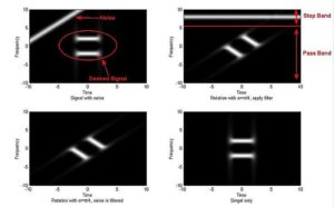
The point of this mathematical manipulation is that it can convert signals into forms that are easier to work with than if left in either the time or frequency domain. For example, FrFTs are increasingly used for handling optical and millimeter-wave communication signals that, frequency-wise, sit close to other interfering signals or electrical noise. It may be possible to apply an FrFT to the signal in a way that converts the band of interfering frequencies into a single frequency that differs from the frequency of interest. This conversion allows a simple filter to remove the problem frequency from the converted signal. Then an inverse FrFT operation can return the resulting signal back to the original form, without the noise. There is an article in Wikipedia on the FrFT that illustrates this use quite well.
One might wonder how electronic circuits can perform an FrFT on an incoming signal. First consider the operation of spectrum analyzers. Prior to the development of FFT in 1965, spectrum analyzers were exclusively swept-tuned instruments. A built-in superheterodyne receiver down-converted a portion of the signal spectrum at the input to the center frequency of a narrow band-pass filter. The instantaneous output power was displayed as a function of time. A voltage-controlled oscillator was used in the superheterodyne section to sweep the center frequency through a range of frequencies, creating the frequency-domain display. The disadvantage in the swept-tuned analyzer was that as particular frequencies were displayed, the over-all spectrum was not active, and short-duration events at the other frequencies could be missed.
Within two years after its rediscovery in 1965, FFT technology found its way into the spectrum analyzer. In conjunction with a receiver and analog/digital converter, the FFT-based frequency analyzer, as in the swept-spectrum instrument, processes a portion of the input signal spectrum. The difference, however, is that the spectrum is not swept. The receiver reduces the sampling rate so the FFT spectrum analyzer can process all the samples. As a result, short-term events are accessed.
Spectrum analyzers found on test benches pretty much all operate according to these principles. In contrast, there is no standard electronic approach for computing an FrFT. Moreover, there are no commercially available test instruments as of this writing that will implement an FrFT. A review of the scientific literature on FrFT work reveals that most researchers don't apply the FrFT in real time. They more typically use a program such as Matlab to calculate the effect of the conversion.
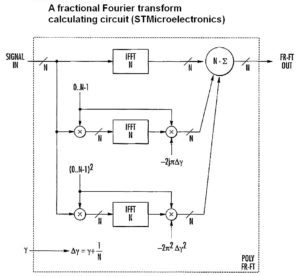
However, there is a great deal of interest in the FrFT for millimeter wave signal processing. It is illustrative to see how research groups are approaching the electronic implementation of FrFT. One example comes from a patent filed by STMicroelectronics Belgium NV. The mathematics underlying the FrFT is quite complex– the starting point is generally to take the FT integral to a non-integer power determined by the chosen FrFT angle. Engineers at STMicroelectronics approached the electronic implementation of the FrFT by expressing the underlying expression as a Taylor series, an infinite sum of terms that are expressed in terms of the function's derivatives at a single point. The patent only mentions a circuit implementing the first three terms of the series, but we might surmise implementations on real ICs probably use more. Each block of the circuit implements one of the Taylor terms. Each block implements an inverse FFT, and all but the first block also implement two multiplications. All the blocks are summed to produce the final result.
The fact that each block in the circuit executes an inverse FFT illustrates the complexity involved in computing the FrFT. It will be interesting to see if the FrFT eventually becomes a function on a test instrument that can be invoked with a pushbutton.
You may also like:
Source: https://www.testandmeasurementtips.com/a-fractional-fourier-transform-yes-there-is-such-a-thing-faq/
0 Response to "Fractional Fourier Transform Continuous in Alpha"
Post a Comment